Polarization Curves: setup, recording, processing and features

Set up your Measurement

Polarization curves are made by making a linear sweep of the sample’s potential over time. In analytical research fields of electrochemistry this technique is called Linear Sweep Voltammetry (LSV), which is the same name PSTrace uses for this technique in Scientific Mode. In Corrosion Mode this technique is labeled Linear Polarization.

Installing the sample

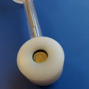
Before the measurement’s parameters will be discussed, the setup for the measurement is described. The sample is installed (see Figure 3.3) in the holder.

The cell is filled with the electrolyte. The cell can be filled with 1 L of solution. Suitable are various salt solutions. Which one is chosen depends on the application and the real environment the sample is exposed to. A common electrolyte is sodium chloride solution (NaCl). The concentrations vary, but a common concentration is 0.5 M NaCl. Conducting solutions like NaCl or KCl are making it easy for electrochemistry to happen, but that also means that corrosion happens more easily.

Low salt concentrations reflect sometimes the behavior of a sample in the real environment better, but they cause an IR-drop. The IR-drop is the part of the applied potential that the working electrode or sample doesn’t feel. This missing potential is caused by the electrolyte between the reference and working electrode acting as an ohmic resistor with the resistance R_u. The IR-drop is calculating by multiplying the flowing current I and R_u according to Ohm’s law.

In 2018 PalmSens released a module for the PalmSens4, which allows an automatic compensation of the IR-drop during the measurement.

Immersing the electrodes

Before or after filling the cell, the counter electrodes are inserted into the cell. Usually both types of counter electrodes, platinum or graphite, will work fine. If nothing special is required, the graphite rods are a good choice. They have a large surface area and are inexpensive. The platinum electrodes are sensitive to mechanical stress, especially the connection between the wire and the sheet, but they are quite chemically inert and will also be resistant to oxidizing solutions, which might attack graphite.

The counter electrodes task is to deliver enough current for the working electrode. When the area of the counter electrode is large enough the capacitive current of the electrode will suffice and only very few chemical changes are caused by the counter electrode. To turn the two counter electrodes in one big one, just short circuit both counter electrodes with a cable.

The working electrode or the sample should be placed in the center opening.

The reference electrode is a bit delicate and it is recommended to read the manual of the reference electrode. When a reference electrode is not used, it should be stored with the frit’s end in 1 M (or higher) KCl. The ItalSens Corrosion set also contains a salt bridge for your reference electrode. The bridge has a fitting top for the reference electrode and the bottom can be covered with a Teflon cap. This cap has a ceramic sand core.

Positioning of the Reference Electrode’s Tip

When measurement solutions have a low salt concentration, they have a high resistance. A high resistance and/or a high current can lead to a significant IR-drop, i.e. there is a difference between the applied potential and the potential felt by the working electrode. In such a situation the salt bridge can decrease the resistance between the reference and working electrode. The bridge is filled with a well-conducting solution, e.g. 0.5 M NaCl, and covered with the Teflon cap. The Teflon cap is placed close to the working electrode to reduce the distance the current travels through high resistance solution.

Placing the Teflon cap close to the working electrode can lead to an artificial crevice formation, so the placement needs to be done carefully. If a well-conducting solution is used, the salt bridge does not need the Teflon cap. However, don’t forget to fix the position of the reference electrode with the ball and socket clamp when using the ItalSens Corrosion Cell Kit.

Gas inlet

The gas inlet is needed if a certain gas needs to be removed or added to the solution. For example, oxygen can be added to reduce diffusion limitation or oxygen can be removed by nitrogen flow to study the reaction in the absence of oxygen. Just connect the gas inlet to your gas source and immerse it in the solution. For most applications a gentle stream of bubbles for 15 minutes will suffice to remove other gases or saturating the solution with a gas.

After connecting all the electrodes to your potentiostat, the cell is ready for the measurements.

Recording Polarization Curves

As previously mentioned to record a polarization curve the technique Linear Polarization (Corrosion Mode) or Linear Sweep Voltammetry (Scientific Mode) needs to be chosen. If a sample’s polarization curve is unknown, all current ranges can be made available, i.e. all current ranges are blue. After the first measurements, current ranges higher than the maximum current should be switched off.

Please keep in mind that the maximum current a PalmSens4 can measure in each current range is 6 times the current range. The lower current ranges allow a better current resolution for lower currents. Unfortunately, the changing of current ranges can induce some artifacts to a measured curve. Should a curve show a spike or a step that can be associated with a current range change, it is advised to only use a single current range for the measurement.

Pretreatment Settings

If no specific potential needs to be applied to the sample before the measurement, the Pretreatment Settings are not important. Check if t deposition and t condition are set to 0 and close this section by clicking on the small arrow.

In the section for the Linear Polarization Settings the t equilibrium is the time that elapses while the starting potential is applied but no values are recorded. This is quite useful to exclude the initial capacitive current of a measurement. The capacitive current is the result of the electrochemical double layer.

Positive or negative charges (depending on the polarization) accumulate at the electrode surface during a potential step. Ions of opposing charge are attracted to the electrode and form a layer in front of the electrode. This form of charge separation is in principle a capacitor and indeed the behavior of an electrode in a solution of inert ions is the same as in a capacitor.

Switching on the cell

Each measurement begins with switching on the cell, which leads to a potential step from the corrosion potential to the set potential for the start. This often leads to a capacitive current which decays exponentially. This is one reason, why often the first 3 to 8 s of the measurement are not used, i.e. the t equilibration is 3 to 8 s. Another reason is that the potentiostat’s auto-ranging has time to choose the proper current range.

E begin and E end are the potentials where you want to start and end your polarization curve. Please note that in the scientific mode the potentials are all versus the reference electrode. In the corrosion mode the potentials are versus the OCP or respectively the corrosion potential E_corr. It is quite common in corrosion research to perform the measurement with potentials in relation to the corrosion potential. This option can be easily controlled manually. If the option isn’t visible on your screen, click on the button with “…” and it will appear (see Figure 5.1).

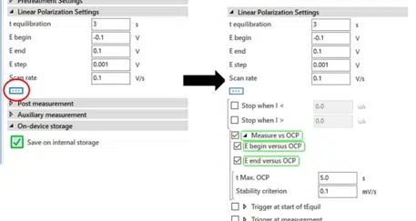
When the boxes are checked the PalmSens will measure the OCP / E_corr before the measurement and set that value as an internal 0. So a -0.1 V in E begin means that the measurement will start 100 mV more cathodic than the E_corr. You can choose the maximum amount of time the measurement of the OCP will take (t Max. OCP). If you expect the OCP to be quite unstable, you want this time be long (up to a few minutes).

If you have already reached a rather stable situation, a few seconds (ca. 5 s) will suffice. The Stability criterion defines a change in mV per s and if the measured change of the E_corr is lower than the Stability criterion, the E_corr measurement is finished. According to literature a change of less than 5 mV per 10 Minutes, so 8.4  µV/s is regarded as a stable state.

Starting and End potentials

The starting and end potentials should be chosen in a way that the measurement starts at least 50 to 100 mV below and ends 50 to 100 mV above the corrosion potential. You can use a broader potential window, if you like. A longer linear part in your Tafel plot will increase the accuracy of the measurement, but more extreme potentials induce more changes to the surface. A broader potential window doesn’t guarantee a longer linear part, because the potential for another reaction, a passivation or diffusion limitation might be reached.

E step defines the potential difference between each point of the measurement, which is the resolution of the measurement. A digital potential cannot perform truly linear changes of the potential. The linear sweep is simulated by small steps of the potential. When E step is increased, the potentiostat has more time for one step, if the scan rate is constant.

This means the potentiostat takes more samples at this potential step and averages them to output a data point. The more values are averaged the more noise is averaged out, because usually noise is equally distributed around the real value. A decrease in E step makes the measurement more noise sensitive, but increases resolution. For most measurements a value between 1 and 5 mV is chosen.

Scan rate

The Scan rate has some critical influences on the measurement. It is from the discussion of E step clear that the Scan rate has the opposing influence on the noise sensitivity. The lower the scan rate, the more samples can be averaged for a data point and more noise is averaged out. More importantly, the Scan rate defines the time scale of the experiment. This can be used to research the kinetics of electrochemical reactions.

For corrosion measurements usually low Scan rates are chosen. This has two reasons.

• First, you want the reactions that are happening to be at a steady state for the corresponding potential.
• Second, you want to measure the current caused by the oxidation and reduction: not the capacitive current, which was discussed previously in the paragraph about t equilibration.

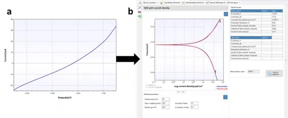
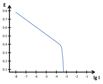
If we are looking at the basic equations for a capacitor, it is easy to see that the capacitive current depends linear on the Scan rate (see chapter Capacitive Current). This isn’t true for digital potentiostats, which work with potential steps during which most capacitive current decays usually a low Scan rate is chosen. According to the literature values of 4 to 20 mV/s should be fine. The raw data will look similar to Figure 5.2 a.

Processing Polarization Curves

After recording the curve you can extract the corrosion current easily from the curve in the Corrosion Mode. Just choose the Corrosion tab above the plot, while the polarization curve is the active curve (blue highlighted in the legend). The polarization curve and an automated fit will appear on the screen. Right to the plot is a small table showing the results of the plot (see Figure 5.2 b).

If the curve of the fit matches the measurement and the values in the table are realistic, you are already done. However, we are offering more options.

The following analysis techniques are supported for the estimation of the corrosion rate based on linear polarization measurements:

• Auto Butler-Volmer fit: Fitting the Butler-Volmer model over an automatically detected range.
• Manual Butler-Volmer fit: Fitting the Butler-Volmer model over a manually selected range.
• Manual Tafel slope fit: Fitting Tafel slopes in the linear regions of the anodic and cathodic slopes.

For all these Options you should note that to achieve an accurate estimation of the corrosion rate it is recommended to use a measurement with at least one linear Tafel slope that ranges over one decade in current density. Additionally, the distance between the Tafel slope and the corrosion potential should at least be 50 mV.

Manual Tafel slope

In the previous chapter the Tafel slopes were discussed already. The option to do a Manual Tafel slope fit allows you to choose a cathodic linear part and an anodic linear part of the curve. Linear fits will be performed on these and a Tafel Analysis is performed. These fits are quite sensitive and easily badly chosen linear parts cause an error of factor 5 or completely unrealistic values. It needs experience to choose the correct linear parts of these curves and see the influence of diffusion limitation.

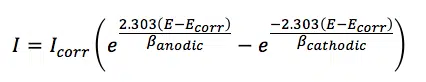
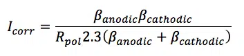
Another approach is the auto Butler-Volmer fit. The Butler-Volmer fit uses the theoretical prediction of a polarization curve according to the Butler-Volmer equation (equation 5.1). It created a relation between applied potential E, the measured current I, the corrosion potential E_corr, corrosion current I_corr and the Tafel slopes for the anodic and cathodic reaction ß_anodic and ß_cathodic, also known as Tafel constants.

This does not require a very long linear range of the polarization curve, because the fit is made to the central part of the polarization curve. Of course, interference with the middle part of the might have an impact on the quality of the fit.

The Manual Butler-Volmer fit allows you to select the range of the curve, which should be used for the fit. This allows you to exclude parts of the curve where other effects than the oxidation or reduction itself have an impact.

The results of these analysis techniques are presented in the Tafel fit results table (Figure 5.3).

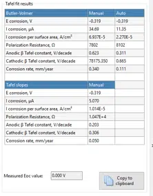
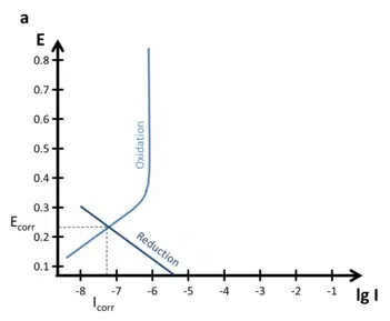
The corrosion potential and the corrosion current have been discussed before. It is quite common to calculate the current density, which is the current per surface, to make measurements between different samples comparable.

Stern-Geary equation

When plotting the current versus the potential the polarization curve is approximately linear close to E_corr (±10 mV). The slope of a line in a voltammogram (current versus potential plot) is a resistance. The slope close to E_corr is called the polarization resistance R_pol. The polarization resistance is of interest for corrosion researchers, because it is inversely proportional to the corrosion current, assuming that the Tafel slopes are constants. This is described by the Stern-Geary equation (equation 5.2).

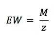
The corrosion rate in mm/year can be calculated according to the standard practice described in the ASTM Standard G 102. To calculate an estimation of corrosion the corrosion current as well as the following material parameters are needed: equivalent weight EW in g/mol, the density ρ in g/cm³, and the sample area A in cm² of the study sample. Combined with a constant (K) defined by the ASTM (3272 mm/(A*cm*year*mol)) this information is used to determine the corrosion rate in mm/year according to equation 5.3.

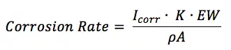
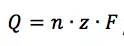
K is the summary of a few constants. Equation 5.3 is derived from Faraday’s law (equation 3.1) by introducing the equivalent weight EW. For an atomic species (so pure metals) the equivalent weight EW is the atomic weight AW divided by the number of electrons needed for conversion z (equation 5.4). AW corresponds here to the more commonly used, molecular weight M.

The equivalent weight EW of alloys is more complex to determine. If an alloy is corroding homogeneously, the EW is the weighted averaged molecular M of the alloy components. The weighting factor is the mole fraction of each component. Many alloys do not dissolve homogeneously. If you want to calculate a corrosion rate for them anyway, you need to measure in which mole fraction the alloy dissolves, for example by investigating the solution in contact with the alloy before and after a corrosion event.

Implications

There are some implications in the corrosion rate and its calculation. One of the most prominent ones is the assumption that the surface corrodes homogeneously. We calculate the converted mass, from that the volume of that mass and that volume we spread evenly across the area of the sample to get the corrosion rate. This is often not true. Events like pitting corrosion appear, alloys corrode faster around phase boundaries, crevices corrode faster, etc. The corrosion rate is still a great parameter to compare the behavior of different materials in certain environments, but the values should be taken with a pinch of salt.

Features of Polarization Curves

Polarization curves often give indications of what is happening at the surface. Diffusion was already discussed before (see chapter Tafel plot and Evans Diagram). It is not always easy to recognize and differentiate between a rather slow reaction and a diffusion limited reaction. Since the sample itself is usually the oxidizing partner, which is available in abundance, diffusion limitation is usually in the reductive part of the polarization curve.

Often the reduction is the reduction of oxygen, which is free diffusing in the solution and thus can be depleted. The effects of a diffusion limitation are visible in Figure 4.2. Unfortunately, the transition is in a real polarization curve from the linear part to the diffusion limited part quite hard to see.

Pitting corrosion can create misleading features as well. The onset is often characterized by a decrease of the Tafel slope, but if pitting corrosion appears already close to the E_corr it is difficult to recognize that pitting corrosion occurs.

The influence of other substances can sometimes be isolated by choosing a different measurement solution or choosing a different electrode. An iron electrode in alkaline sulfide solution will show sulfide oxidation next to the iron oxidation current. This can be identified with a platinum electrode, because platinum does not oxidize itself, so all measured current can be attributed to sulfide.

Polarization Curves of Thick and Thin Passivation Films

Quite interesting polarization curves are the ones of passive alloys or metals. There are two types of passive metals: thick and thin film. A thick film metal shows resistance to corrosion even when there is a driving force for corrosion (sufficient potential). The Evan’s diagram of such a system is shown in Figure 5.4 a.

Other metals or alloys show a decrease in the current density, if the potential is increased towards anodic potentials. These metals form a thin protective layer after reaching a critical potential. An Evan’s diagram can be seen in Figure 5.4 b.

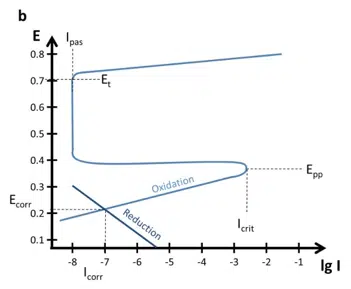
Important parameters are the primary passivation potential E_pp, the critical passivation current I_crit, the passive current I_pas, and the transmission potential E_t. At E_pp and I_crit the oxidation is strong enough to form a dense layer that protects the sample. The current drops to I_pas instead of the expected current predicted by a Tafel plot.

At the potential E_t oxidative processes can happen through the thin film und will quite likely lead to destruction of the protective layer. This behavior can cause quite some interesting effects on the polarization curves (see Figure 5.4 b). The processes below E_pp cause a polarization curve as we know it from the previous chapters, but the anodic part would not show a Tafel behavior for potentials above E_pp.

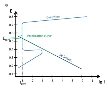
If the cathodic reaction has its intersection with the anodic reaction in the area of the passivation (above E_pp below E_t), the corrosion current I_corr is significantly lower than without passivation see Figure 5.5 a. If you want to estimate I_corr without the passivation for this figure, just extend the linear part of the oxidation curve below E_pp until you have the intersection with the reduction. That I_corr would be in the µA range.

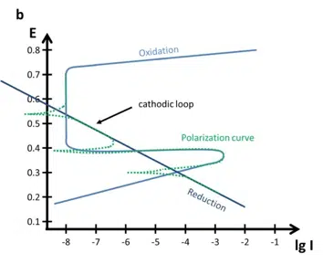
A more complex polarization curve occurs, if the reduction Tafel plot and the oxidation Tafel plot have multiple intersections as shown in Figure 5.5 b. Despite a more anodic potential suddenly a reductive current appears, due to the fact that the surface is now passive. In such a case the E_corr of the sample is usually the highest or lowest of the three intersections.

Film formation can also be studied using cyclic polarization also known as cyclic voltammetry. The film formation can be observed during an anodic scan followed by a cathodic scan, which then shows the cathodic loop. Or it would be possible investigate the repassivation potential.

If during the anodic scan the film was destroyed due to very high anodic potentials, the film won’t be reestablished immediately. The potential needs to drop below a certain threshold, the repassivation potential, for the formation of a stable protective layer.

Pitting and Crevice corrosion

These are two quite complex topics, which are explained here briefly. Both are local processes, which can lead to a corrosion of the whole surface.

Pits are small spots where corrosion appears. Instead of spreading wide most of them penetrate the surface and then spread. This way a coating is undermined. During an anodic scan a sudden increase in the Tafel slope might indicate corrosion pitting. If this high Tafel slope is used for calculating the corrosion rate and the whole surface area of the sample is used, the corrosion rate is significantly underrated.

Passivated metals often show metastable pitting corrosion before the real pitting corrosion starts. The metastable pitting corrosion creates some current spikes in the polarization curve, which can be easily confused with noise. These spikes are the result of pit formation and these pits passivate again, so the pits have only a short lifetime.

Pits of a certain depth and crevices have the same problem. The diffusion inside the pits and crevices is quite limited. Mechanisms developed for steel corrosion are widely accepted as the foundation for the general process of local corrosion. First reduction of oxygen is happening everywhere at the surface, but the oxygen in the crevice is depleted after a while and diffusion is too slow to replenish significant amounts.

This means that inside the crevice the oxidation of the metal occurs, but the whole surface area is reducing oxygen. This separation of anode and cathode is the initial step that triggers local corrosion. The electrons taken from the crevice anode are compensated by a flux of chloride ions into the crevice.

Metal complexes are formed inside the crevice, which are hydrolyzed and releasing protons this way. The pH in the crevice is dropping and thus the solution inside the crevice becomes more aggressive. This process is self-sustaining creating a critical crevice solution (CCS), which is strong enough to remove the passive film.

Starter kit

A great way to create your own Polarization Cruves, is using one of the starter corrosion kits.