Warburg impedance
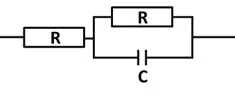
It was observed that some effects occur in EIS that can’t be modeled with classic electronic components, so new components were introduced. One of them is the Warburg impedance. The Randles circuit (Figure 6.7) is quite close to an electrochemical experiment. The solution resistance Rsol is the serial resistor. All current needs to go through the solution.
The current can go through the interface of the working electrode by capacitive current caused by the electrochemical double layer, represented by the double-layer capacity Cdl, or by Faraday current caused by an electrochemical reaction, which requires an electron transfer and so needs to go through the charge transfer resistance Rct.
Up to here, the expected EIS would be a semi-circle just as for the simplified Randles circuit. If a free diffusing species is converted at the electrode, this behavior isn’t observed. At low frequencies oxidizing or reducing potentials are held long enough that depletion of the species in front of the electrode becomes relevant. The depletion of species in front of electrodes is well understood and described by the Cottrell equation.
Due to the lack of species in front of the electrode, fewer species are converted and less current flows while the same potential is applied. During an EIS measurement, this is measured as an increase in impedance. This increase is represented by the Warburg Impedance W, which is a virtual electronic component only used to make equivalent circuits for electrochemical experiments. The Warburg element’s impedance is calculated by
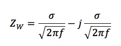
Where ZW is the impedance of the Warburg element and σ is the Warburg coefficient also known as AW. It has the unit Ω/s½ and can be extracted from measurement data or it can be calculated according to
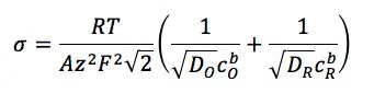
Where R and F are the Gas and Faraday constant, D is the diffusion coefficient and cb the concentration of the species in the bulk. The indices O and R indicate the oxidized and reduced species.
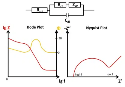
The Warburg Impedance is visible in the Nyquist plot as a straight line with a 45 ° angle to the abscissa. As mentioned before the depletion has a significant effect on the impedance at lower frequencies. When it becomes visible depends on the double-layer capacitance. A schematic representation of a full electrochemical system’s EIS is shown in Figure 6.8.
As mentioned before, the Randles circuit contains a free diffusing species. This is typical for analytical electrochemistry, but doesn’t have to be true for corrosion experiments. An example where this equivalent circuit works quite nicely is a non-porous electrode (e.g. platinum disc electrode) and a reversible redox couple in solution (e.g. ferrocyanide and ferricyanide). Two examples are shown in Figure 6.9.
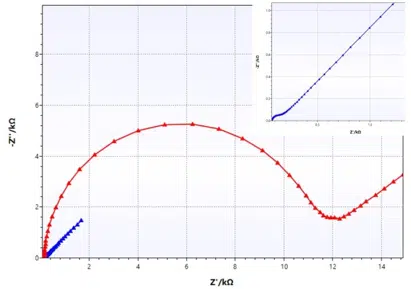
The platinum electrode (blue curve) has a very low charge transfer resistance, leading to a dominance of the Warburg impedance at very low resistances, while the carbon electrode by ItalSens (red curve) shows a significantly higher charge transfer resistance, leading to the expected semi-circle.
These two examples are found in your PSData folder after the installation of PSTrace. There are many different Equivalent circuits and often several ones can deliver a good fit for the spectra. It is important that one tries to find a circuit where every component represents a real process or an element of the electrochemical system. It is good practice to try to keep the number of elements in the circuit low.
Articles
Equivalent circuit fitting for corrosion measurements
In this section of the handbook the Warburg Impedance and the Constant Phase Element (CPE) are introduced, which represent electrochemical effects with no corresponding real electronic components. Furthermore, some equivalent circuits for typical corrosion systems are presented.